AE 07 – Meet the Lemurs

Application exercise

This week we’ll be working with data from the Duke Lemur Center, which houses over 200 lemurs across 14 species – the most diverse population of lemurs on Earth, outside their native Madagascar.

Lemurs are the most threatened group of mammals on the planet, and 95% of lemur species are at risk of extinction. Our mission is to learn everything we can about lemurs – because the more we learn, the better we can work to save them from extinction. They are endemic only to Madagascar, so it’s essentially a one-shot deal: once lemurs are gone from Madagascar, they are gone from the wild.

By studying the variables that most affect their health, reproduction, and social dynamics, the Duke Lemur Center learns how to most effectively focus their conservation efforts. And the more we learn about lemurs, the better we can educate the public around the world about just how amazing these animals are, why they need to be protected, and how each and every one of us can make a difference in their survival.

Source: TidyTuesday

Packages and Data

First let’s load the packages we’ll need.

library(tidyverse)
library(infer)

And then load the data.

lemurs <- read_csv("lemurs.csv")

Although our dataset contains 54 variables, we’ll only focus on the following 3:

variable	type	description
taxon	char	Taxonomic code: in most cases, comprised of the first letter of the genus and the first three letters of the species; if taxonomic designation is a subspecies, comprised of the first letter of genus, species, and subspecies, and hybrids are indicated by the first three letters of the genus.
sex	char	M=male. F=Female. ND=Not determined
weight_g	double	Animal weight, in grams. Weights under 500g generally to nearest 0.1-1g; Weights >500g generally to the nearest 1-20g.

Count the Lemurs

Our dataset includes three species of lemur, shown in the taxon variable using the following taxonomic codes:

Taxon	Latin name	Common name
EMON	Eulemur mongoz	Mongoose lemur
ERUB	Eulemur rubriventer	Red-bellied lemur
LCAT	Lemur catta	Ring-tailed lemur

lemurs |>
  count(taxon)

# A tibble: 3 × 2
  taxon     n
  <chr> <int>
1 EMON     97
2 ERUB     23
3 LCAT    224

Question 1

Summarize the results of the code chunk above, using the table above to interpret the taxonomic code.

Add response here

Mean Lemur Weights

Let’s investigate the weight of these lemurs. Since we know that our dataset includes three different species of lemur, we might suspect that different species will be different sizes. So lets separate our visualization using the taxon variable:

lemurs |>
  ggplot( aes(x=weight_g, fill = taxon) ) +
  geom_boxplot()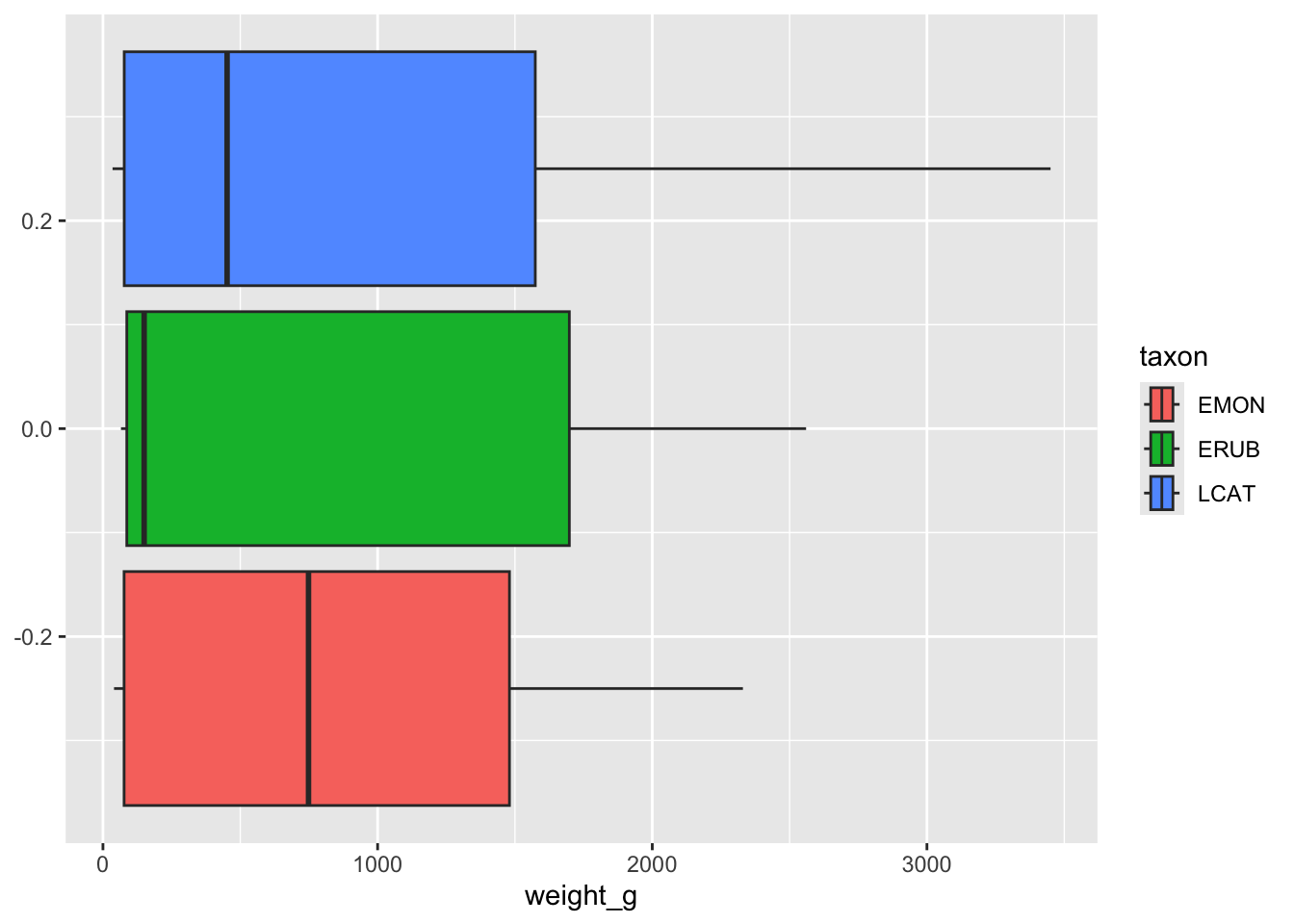

Question 2

Summarize your observations of these box plots.

Add response here

Ring-Tailed Lemurs

Let’s focus specifically on ring-tailed lemurs by using filter to create a new data set that only contains lemurs with taxon equal to “LCAT”.

lemurs_rt <- lemurs |>
  filter( taxon == "LCAT" )

Mean Weight

Now let’s calculuate the mean value of the variable weight_g. Notice that we are saving the result of this calculation in the variable called obs_stat_mean_rt so that we can refer to it later.

obs_stat_mean_rt <- lemurs_rt |>
  specify(response = weight_g) |>
  calculate(stat = "mean")

obs_stat_mean_rt

Response: weight_g (numeric)
# A tibble: 1 × 1
   stat
  <dbl>
1  924.

Question 3

Write a sentence or two summarizing and interpret the results.

Add response here

Confidence Interval

Now let’s calculate, visualize, and interpret a 95% bootstrap confidence interval.

Step 1: Construct a bootstrap distribution. Since there is a generate() step, you should set a seed value before running. Add the line at the top set.seed(123) and change reps value to 1000 to create your bootstrap confidence interval.

boot_dist_mean_rt <- lemurs_rt |>
  specify(response = weight_g) |>
  generate(reps = 1000 , type = "bootstrap") |>
  calculate(stat = "mean")

Step 2: Visualize your sample distribution.

visualize(boot_dist_mean_rt)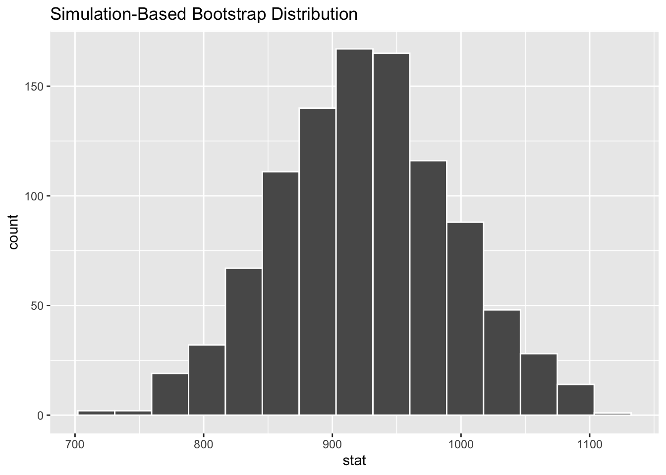

Question 4

Based on this histogram, what’s your estimate for the 95% confidence interval?

Add response here

Step 3: Find the confidence interval precisely.

ci_95_mean_rt <- boot_dist_mean_rt |>
  get_confidence_interval(
    point_estimate = obs_stat_mean_rt, 
    level = 0.95
  )

ci_95_mean_rt

# A tibble: 1 × 2
  lower_ci upper_ci
     <dbl>    <dbl>
1     795.    1060.

Question 5

How does this precise interval compare to your estimate from above?

Add response here

Step 4: Visualize the confidence interval, overlaying it on the bootstrap distribution.

visualize(boot_dist_mean_rt) +
  shade_confidence_interval(endpoints = ci_95_mean_rt)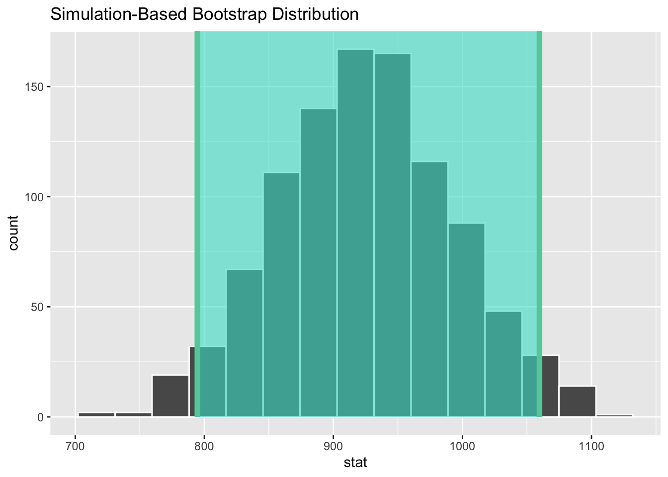

Question 6

Summarize and interpret your findings.

Add response here

Mongoose Lemurs

What happens if we look at a different species? Repeat the above analysis for Mongoose Lemurs.

Start by using filter to create a new data set that only contains Mongoose lemurs.

To Do

Fill in the blank in the code chunk below to create a new dataset that only includes Mongoose lemurs. Then change eval: false to eval: true before rendering.

lemurs_m <- lemurs |>
  filter( --- )

Mean Weight

Calculate the mean value of the variable weight_g and save the result of this calculation in the variable called obs_stat_mean_m so that we can refer to it later.

obs_stat_mean_m <- lemurs_m |>
  specify(response = weight_g) |>
  calculate(stat = "mean")

obs_stat_mean_m

Question 7

Run the above code (by changing eval: false to eval: true. What is the mean weight of our sample of Mongoose lemurs?

Add response here

Confidence Interval

Now we want to calculate, visualize, and interpret a 95% bootstrap confidence interval.

To Do

In the code chunk below, add a set.seed() line and change the number of reps to something reasonable. Remember to change eval: false to eval: true before rendering.

boot_dist_mean_m <- lemurs_m |>
  specify(response = weight_g) |>
  generate(reps = 10 , type = "bootstrap") |>
  calculate(stat = "mean")

Visualize your sample distribution.

visualize(boot_dist_mean_m)

Find the confidence interval precisely.

To Do

Fill in the blank in the code chunk below to specify what confidence level you want.

ci_95_mean_m <- boot_dist_mean_m |>
  get_confidence_interval(
    point_estimate = obs_stat_mean_rt, 
    level = ---
  )

ci_95_mean_m

Visualize the confidence interval, overlaying it on the bootstrap distribution.

visualize(boot_dist_mean_m) +
  shade_confidence_interval(endpoints = ci_95_mean_m)

Question 8

Summarize and interpret your findings.

Add your response here