library(tidyverse)
library(tidymodels)

fish <- read_csv("fish.csv")AE 05 – Modeling Finnish Fish
Application exercise
For this application exercise, we will work with a data set that contains measurements of fish caught in lake Laengelmavesi in southwestern Finland.
The data dictionary is below:
| variable | description |
|---|---|
species |
Species name of fish |
weight |
Weight, in grams |
length_body |
Length from nose to start of tail, in cm |
length_notch |
Length from nose to tail notch, in cm |
length_tail |
Length to end of tail, in cm |
height |
Height, in cm |
width |
Width, in cm |
Visualizing Weight and Height
The question we want to investigate is whether there is relationship between the weights and heights of fish. We start by making a scatterplot to visualize the data.
ggplot(fish, aes(x = height, y = weight)) +
  geom_point() +
  geom_smooth(method = "lm", se = FALSE) +
  labs(
    title = "Weights vs. heights of fish",
    x = "Height (cm)",
    y = "Weight (gr)"
  )
Note that in the code chunk above, the line with geom_smooth draws the linear regression line for us.
One of the reasons why we want to see the linear regression line is that it can help us make predictions. Based on the graph alone, what do you predict would be the weight of a fish that has a height of 8cm? 15cm? 20cm?
Model fitting
Now lets make our linear model more precise by finding the actual equation for the line. As we saw in class, we can calculate the coefficients that we need to describe the line with the following summary statistics.
fish |>
  summarize( mean_x = mean(height),
             sd_x = sd(height),
             mean_y = mean(weight),
             sd_y = sd(weight),
             r = cor(height, weight)
  )
# A tibble: 1 × 5
mean_x sd_x mean_y sd_y r
<dbl> <dbl> <dbl> <dbl> <dbl>
1 12.1 4.47 448. 285. 0.954Recall from class that the equation for the linear model is \[ \hat{y} = b_0 + b_1 \hat{x} \]
where \[ b_1 = r \left ( \frac{ s_y}{s_x} \right ) \] and
\[ b_0 = \bar{y} - b_1 \bar{x} \]
A Shortcut!
It turns out that R can generate the linear model automatically. The following code chunk demonstrates how to do this. In case you’re curious parsnip refers to an R package designed to simplify model fitting.
linear_reg() |>
  fit(weight ~ height, data = fish)
parsnip model object
Call:
stats::lm(formula = weight ~ height, data = data)
Coefficients:
(Intercept) height
-288.42 60.92 Adding a third variable
As we know from our pengiun friends, species can sometimes be a confounding variable. Does the relationship between heights and weights of fish change if we take into consideration species?
ggplot(fish,
       aes(x = height, y = weight)) +
  geom_point() +
  geom_smooth(method = "lm", se = FALSE) +
  labs(
    title = "Weights vs. heights of fish",
    x = "Height (cm)",
    y = "Weight (gr)"
  )
`geom_smooth()` using formula = 'y ~ x'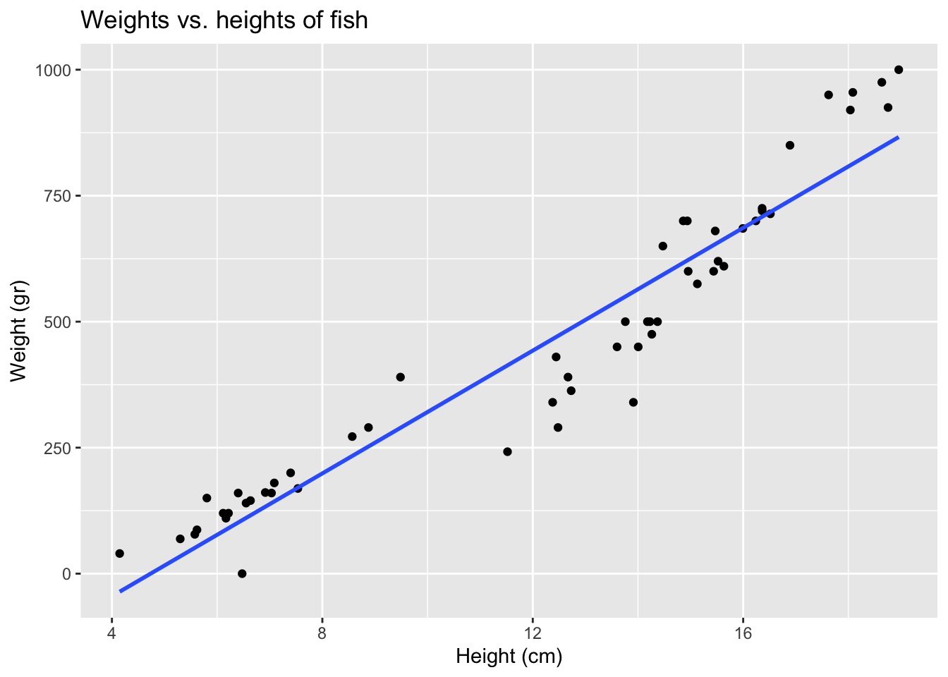
Challenge!
Once you see that we really need two separate linear models for the two different species, we can reproduce our analysis above by first filtering by species. The two species in this data set are “Bream” and “Roach”