Inference for Single Proportion
Chapter 16
Looking Ahead
We will take a closer look at inference methods in different contexts:
- Ch 16: Single Proportion
- Ch 17: Two Proportions
- Ch 18: Two-way tables (multiple proportions)
- Ch 19: Single Mean
Recall our Hypothesis Testing Framework
State the null and the alternative hypotheses
Choose a sample, collect and analyze the data
How likely is it to see data like what we observed, if the null hypothesis were true?
If very unlikely, we reject the null hypothesis. Otherwise, we cannot reject.
p-value
p-value is a probability – how likely is it to see our observation if the null hypothesis is true?
Finding the p-value
- If conditions for Central Limit Theorem are met, can use a mathematical model, i.e. normal curve - find z-scores, etc.
- If conditions for Central Limit Theorem are not met, use simulation methods, i.e. bootstrapping or randomization
Mathematical Model
Needed Conditions
The sampling distribution \(\hat{p}\) based on a sample size \(n\) from a population with a true proportion \(p\) is nearly normal if:
Sample’s observations are independent - roughly: observations do not impact another observations
Success-failure condition – we expect to see at least 10 successes and 10 failures.
- \(np \geq 10\) and \(n(1-p) \geq 10\)
Standard Error Formula (new)
If conditions are met then distribution of \(\hat{p}\) is nearly normal with variability given by the standard error
\[ SE = \sqrt{ \frac{p(1- p)}{n}} \] Note we (usually) don’t know \(p\) (it’s the population parameter) so we use our best guess for \(p\) intead:
- For hypothesis testing, use \(p_0\) (null hypothesis)
- For confidence intervals, use \(\hat{p}\)
Confidence Interval
\[ \mbox{point estimate} \pm z^\ast * SE \]
\(z^\ast * SE\) is the margin of error
\(z^\ast\) is determined by the desired confidence level.
Confidence Level
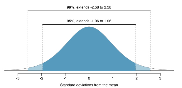
95% confidence level means \(z^\ast = 1.96\)
Example: confidence interval
In survey of 3290 Portland residents, 48.3% of respondents say that homelessness is Portland’s greatest challenge.
- Are CLT conditions met?
- Are observations independent? Yes - random sample
- Success/failure? Yes
- \(np = 3290*0.483 = 1589 \geq 10\)
- \(n(1-p) = 3290 * (1 - 0.483) = 1701 \geq 10\)
Example: confidence interval
In survey of 3290 Portland residents, 48.3% of respondents say that homelessness is Portland’s greatest challenge.
\[ SE = \sqrt{ \frac{p(1- p)}{n}} = \sqrt{ \frac{ 0.483(1-0.483)}{3290}} = 0.009 \] Margin of error \[ p^\ast \times SE = 1.96\times 0.009 = 0.018 \]
Example: confidence interval
In survey of 3290 Portland residents, 48.3% of respondents say that homelessness is Portland’s greatest challenge.
We are 95% confident that the true proportion of Portlanders who agree that homelessness is the city’s greatest challenge
\[ 0.483 \pm 0.018 \]
Hypothesis Test for single proportion
Z-score tells us how the sample proportion (\(\hat{p}\)) differs from the hypothesized proportion (\(p_0\))
\[ Z = \frac{ \hat{p} - p_0}{SE} = \frac{ \hat{p} - p_0}{\sqrt{p_0(1-p_0)/n}} \]
Example
Supporters of ballot measure that would impose stricter regulations on payday lenders commissioned a survey that asked 826 random voters if they supported such a measure. The survey found that 51% of respondents said they did support it. Is there convincing evidence to say that voters support this measure?
Example: hypotheses
Null hypothesis: voters are indifferent (neither support nor oppose) \[ p_0 = 0.5 \]
Alternative hypothesis: voters support \[ p_0 > 0.5 \]
Example: conditions
- independent
- success/failure
- \(np = 825*0.5 = 413 \geq 10\)
- \(n(1-p) = 825*0.5 = 413 \geq 10\)
Example: standard error
\[ SE = \sqrt{ \frac{ p_0(1-p_0)}{n}} = \sqrt{ \frac{0.5(1-0.5)}{826}} = 0.017 \]

Example: Z-score
\[ Z = \frac{ \hat{p} - p_0}{SE} = \frac{ 0.51 - 0.50}{0.017} = 0.59 \]
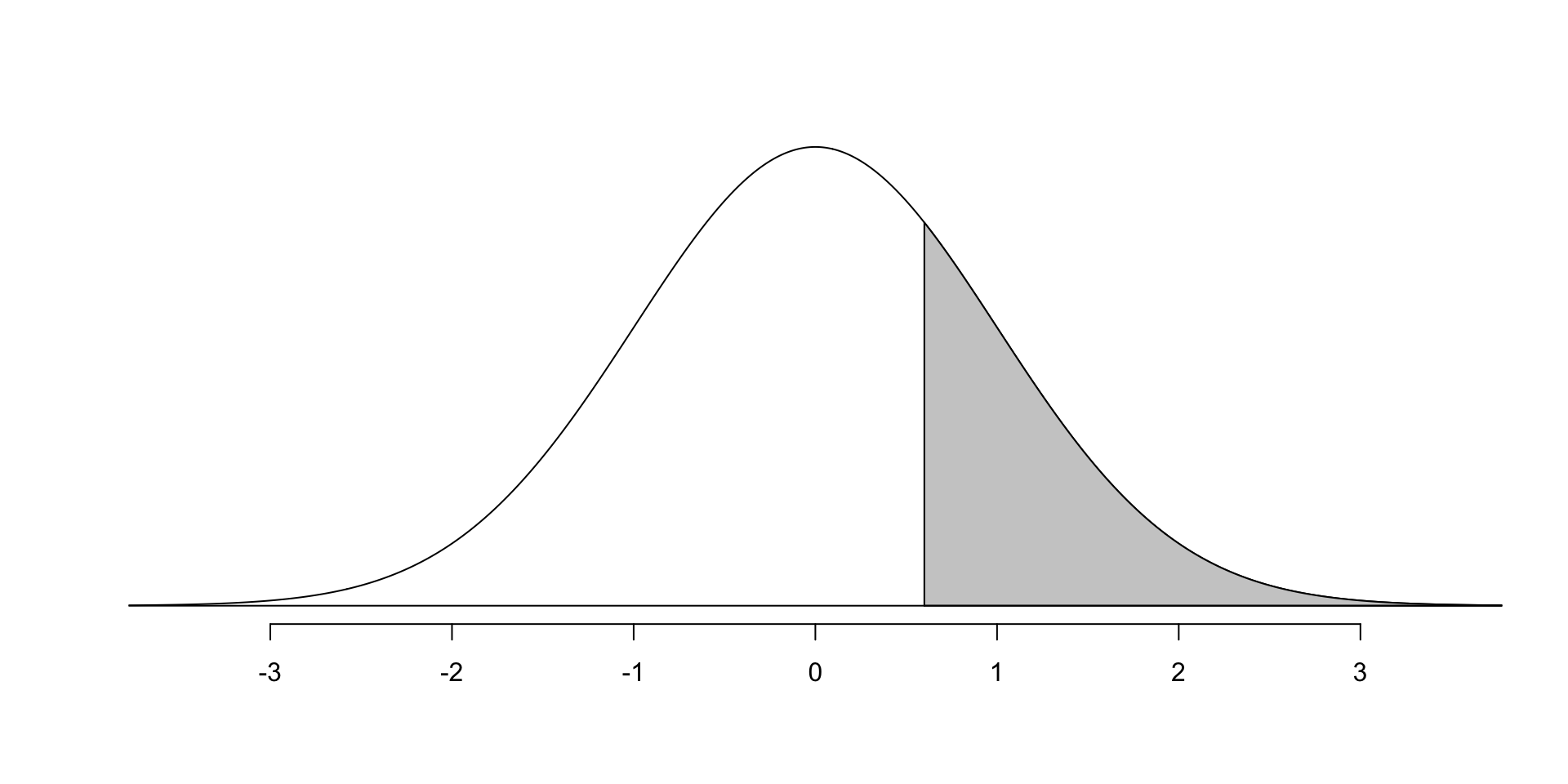
Example: find p-value

Because p-value is larger than 0.05, we do not reject \(H_0\). There is not convincing evidence that there is support for this measure.
What if conditions for CLT are not met?
Independence?
need more advanced methods (beyond scope of our class)
Small sample size?
Use simulations – next time!