Exploring numerical data

Chapter 5

Chris Hallstrom

University of Portland

In groups

Today’s homework: section 5.10, #1, 2, 5a,b

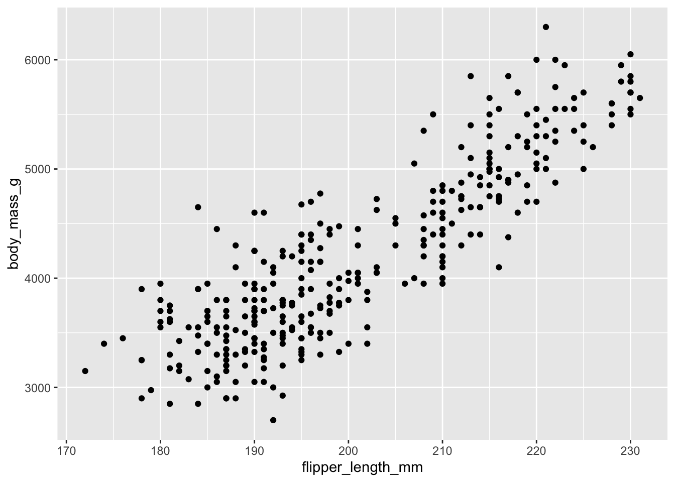
Scatterplots

Compare two numerical variables

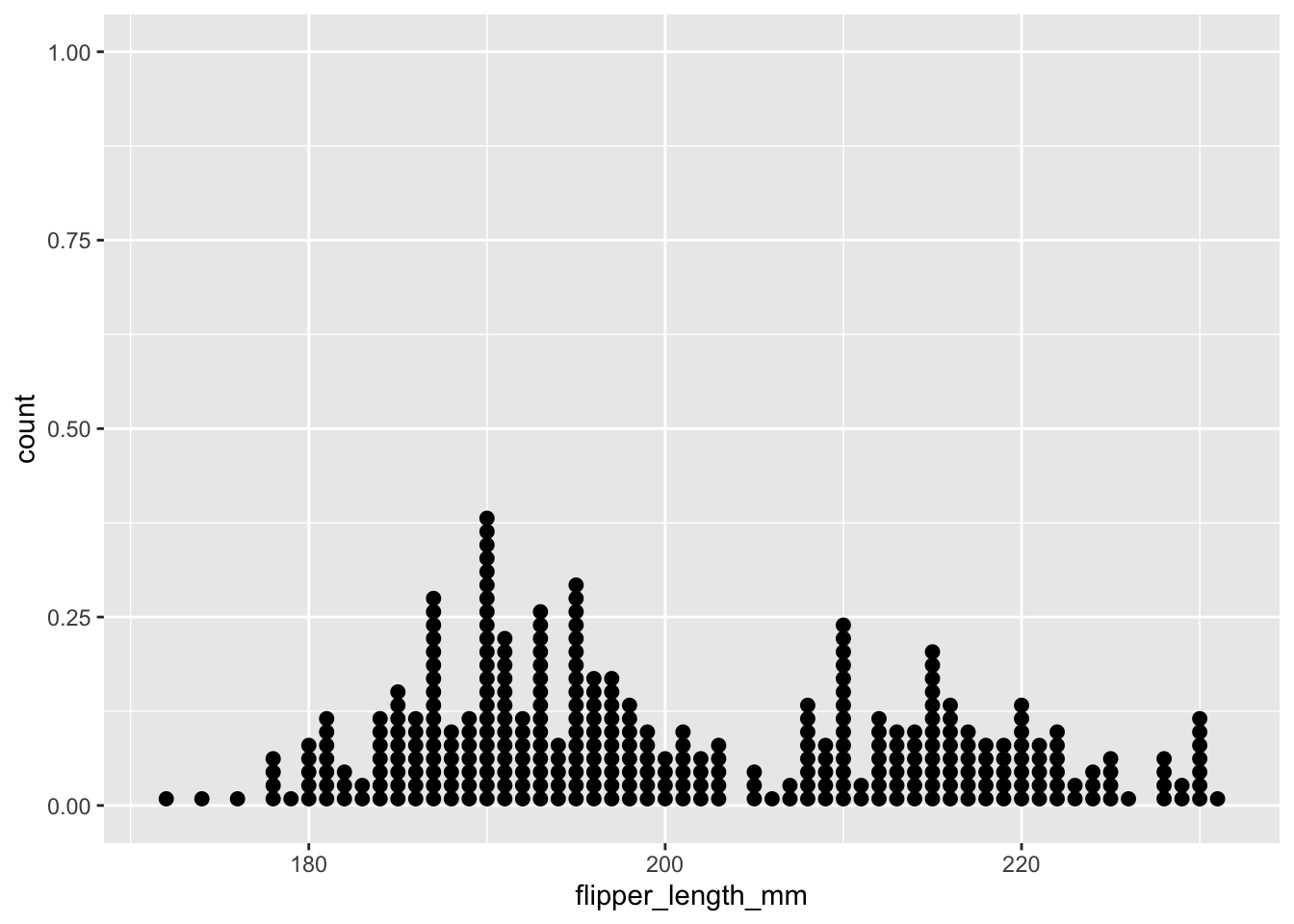
Dot Plot

Visualize the distribution of one numerical variable

ggplot(data = penguins, 
       mapping = aes(x = flipper_length_mm)) +
  geom_dotplot(dotsize=0.75, binwidth=1)

flipper_length_mm

penguins |> count(flipper_length_mm) |> print(n=20)

# A tibble: 56 × 2
   flipper_length_mm     n
               <int> <int>
 1               172     1
 2               174     1
 3               176     1
 4               178     4
 5               179     1
 6               180     5
 7               181     7
 8               182     3
 9               183     2
10               184     7
11               185     9
12               186     7
13               187    16
14               188     6
15               189     7
16               190    22
17               191    13
18               192     7
19               193    15
20               194     5
# ℹ 36 more rows

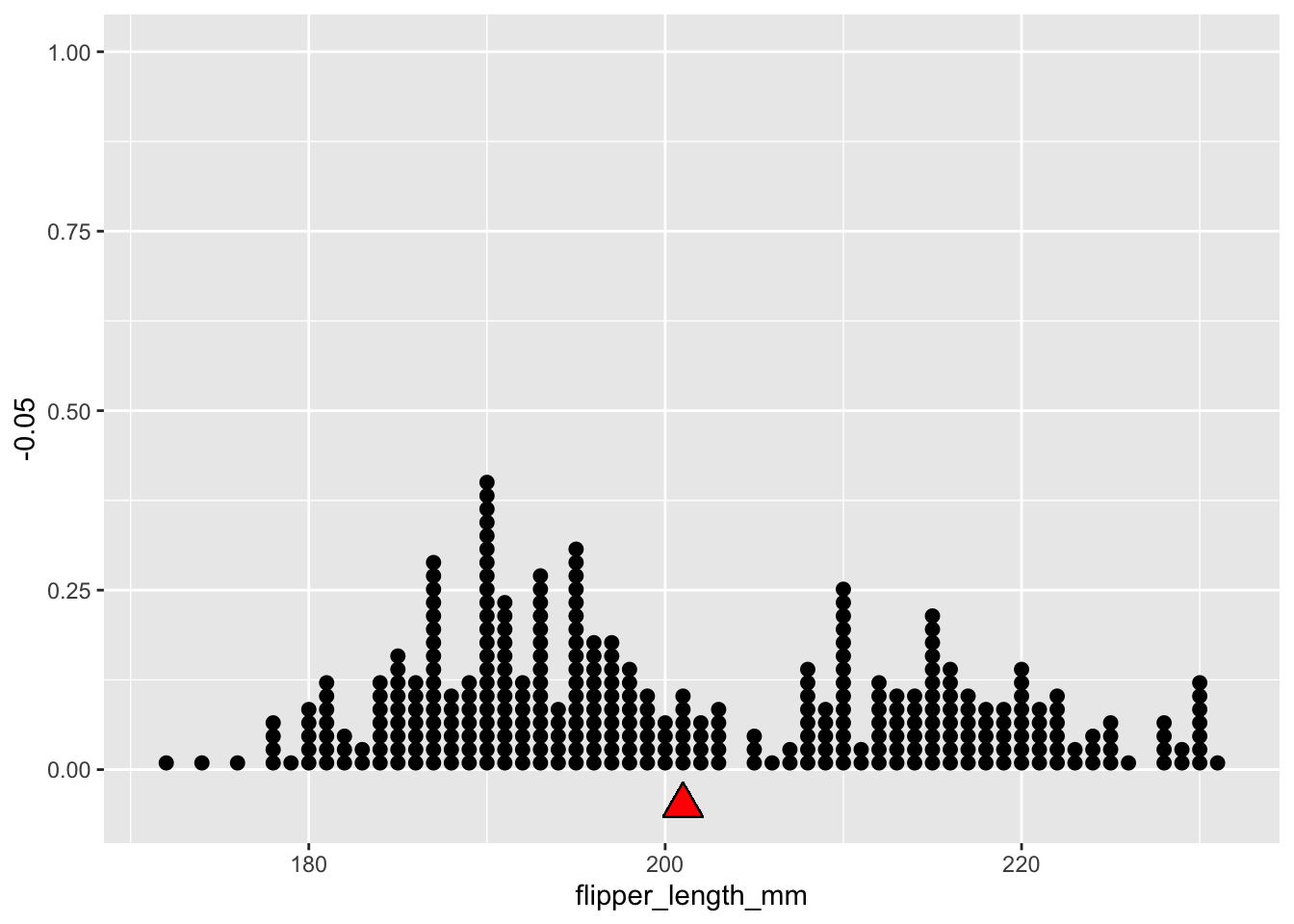
Mean (average) flipper length?

mean(penguins$flipper_length_mm, na.rm = TRUE)

[1] 200.9152

penguins |>
  summarize( mean = mean(flipper_length_mm, na.rm = TRUE))

# A tibble: 1 × 1
   mean
  <dbl>
1  201.

Visualize the Mean

A measure of center of a distribution.

Calculuating the Mean

Sample mean \(\overline{x}\)

\[ \overline{x} = \frac{ x_1 + x_2 + x_3 + \ldots + x_n}{n} \]

Population mean \(\mu\) (Greek letter “mu”) \[ \overline{x} \approx \mu \]

Question: what is the average age of the people in this room?

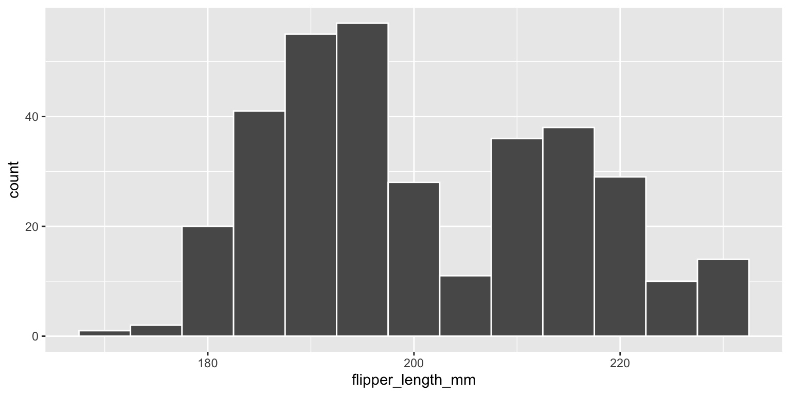
Histogram

ggplot(data = penguins, 
       mapping = aes(x = flipper_length_mm)) +
  geom_histogram(binwidth = 5, color="white" )

This distribution is bimodal and right skewed

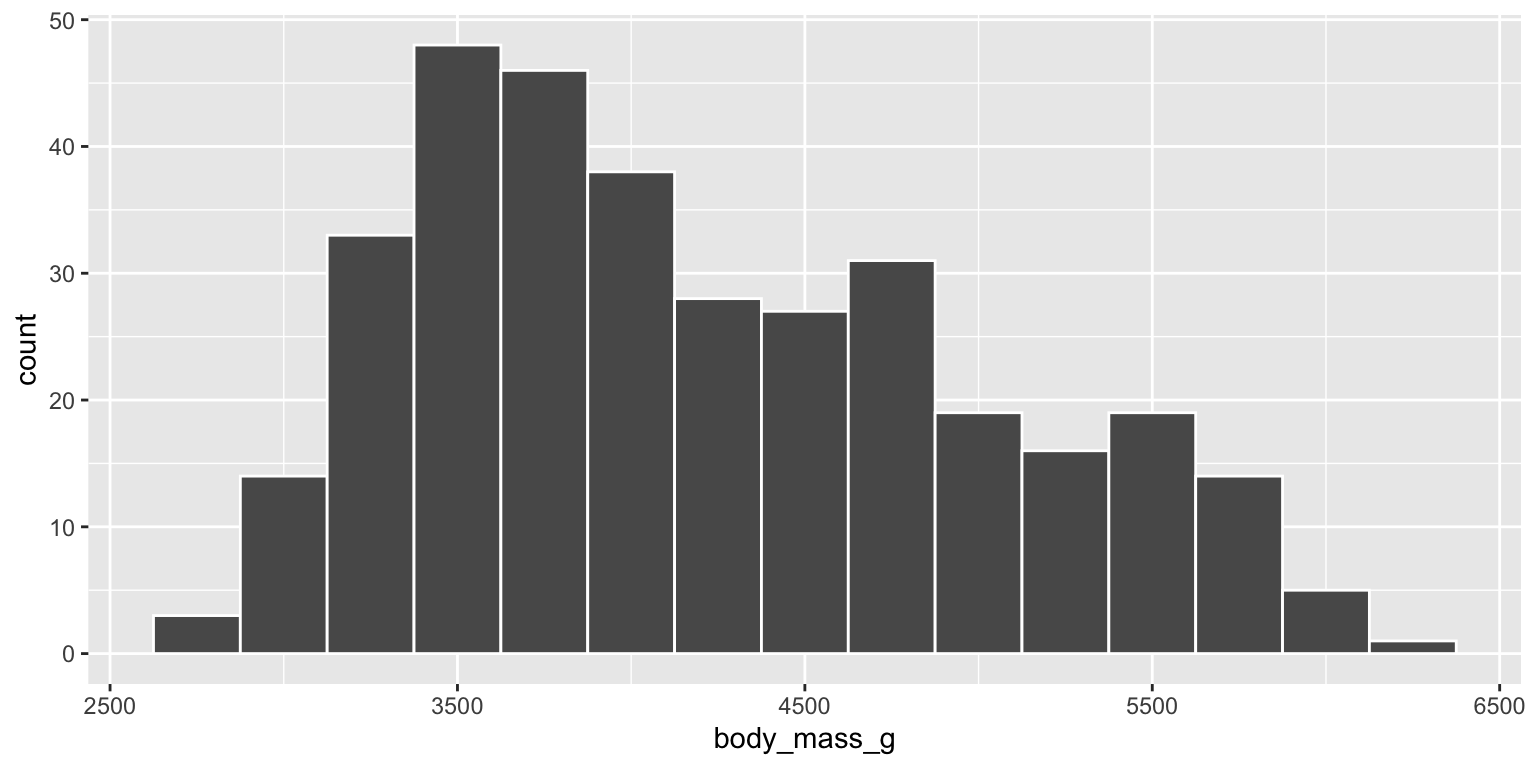
Body Mass

ggplot(data = penguins, 
       mapping = aes(x = body_mass_g)) +
  geom_histogram(binwidth = 250, col="white")

This distribution is unimodal and right skewed

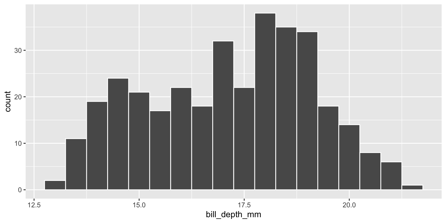
Bill Depth

ggplot(data = penguins, 
       mapping = aes(x = bill_depth_mm)) +
  geom_histogram(binwidth = 0.5, col="white")

This distribution is bimodal and right skewed

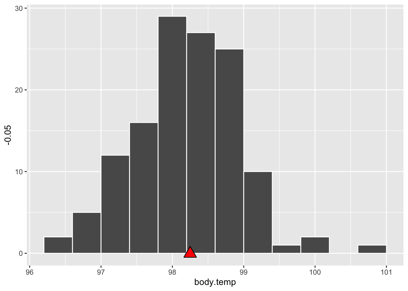
Mean (average) Body Temperature

What do you think it is?

Mean (average) Body Temperature

mean(thermometry$body.temp)

[1] 98.24923

Variance

Measure of variation or how spread out distribution is. It’s the average squared distance from the mean.

Sample variance is \(s^2\)

where s is the sample standard deviation \[ s = \sqrt{ \frac{ \sum_{i=1}^n (x_i - \overline{x})^2 }{n-1}} \]

Population variance: \(\sigma^2\) (Greek letter “sigma”)

Standard Deviation

s is the sample standard deviation. Represents the typical deviation from the mean \[ s = \sqrt{ \frac{ \sum_{i=1}^n (x_i - \overline{x})^2 }{n-1}} \]

Empirical Rule

Typically, about 68% of the data (observations) lie within one s.d. of the mean.

About 98% of the data lie within two s.d. of the mean.

These percentages are not hard and fast rules!

Body Temperature

thermometry |>
   summarize( mean = mean(body.temp), sd = sd(body.temp))

      mean        sd
1 98.24923 0.7331832

Using the empirical rule, about 68% of observations lie in what range of temperatures?

IQR

summary(thermometry$body.temp)

   Min. 1st Qu.  Median    Mean 3rd Qu.    Max. 
  96.30   97.80   98.30   98.25   98.70  100.80