Confidence Intervals with Bootstrapping

Chapter 12

In groups

• Discuss Homework: Chapter 12, #1, 3, 7

Confidence Intervals

Goal is to estimate a population parameter

\(p\) – true value of a parameter (usually unknown)

\(\hat {p}\) – sample statistic

How confident can we be that the value of \(\hat {p}\) is close to \(p\)?

Case Study

A medical consultant helps guide transplant patients through all the stages of surgery. Out of a total of 62 clients, only 3 had complications:

\[ \hat{p} = 3/62 = 0.048 \]

Consultant claims that her rate is less than the national rate of 10%.

Question – how confident can we be that \(p\) is less than the national rate of 0.1?

Distributions

We know that there’s some variation in the data. But how much?

If this particular consultant had another 62 clients, how many of them might have complications?

This is similar to what we did last week.

We need to know the sampling distribution.

Two Steps

1. Find the distribution

2. Use the distribution to find confidence interval

Step 1 – Find Sampling Distribution

• Determine with math!
  We’ll come back to this in Chapter 13.

• Bootstrapping!
  Use the observed proportion to construct a new population and resample from that.

• Someone else gives this to us. (e.g. see Chapter 12 homework)

Bootstrap

Want 62 new outcomes each with a 0.048 chance of having a complication. Put 62 marbles in a bag

• 3 labeled “C”
• 59 labeld “NC”

1. pick a marble
2. note outcome
3. put back into bag (sample with replacement)
4. repeat

Resample #1

“NC”, “NC”, “NC”, “NC”, “NC”, “C”, “NC”, “C”, “NC”, “NC”, “NC”, “NC”, “NC”, “NC”, “NC”, “NC”, “NC”, “NC”, “C”, “NC”, “NC”, “NC”, “NC”, “NC”, “NC”, “NC”, “NC”, “NC”, “NC”, “NC”, “NC”, “NC”, “NC”, “NC”, “NC”, “NC”, “NC”, “NC”, “NC”, “NC”, “NC”, “NC”, “NC”, “NC”, “NC”, “NC”, “NC”, “NC”, “NC”, “NC”, “NC”, “NC”, “NC”, “NC”, “NC”, “C”, “NC”, “NC”, “NC”, “C”, “NC”, “NC”

Complications: 5/62 = 0.081

Resample many times to get sample distribution

set.seed(25) 

boot_dist_donor <- organ_donor |>
  specify(response = outcome, success = "complication") |>
  generate(reps = 1000, type = "bootstrap") |>
  calculate(stat = "prop")

Visualize

boot_dist_donor |>
  ggplot( aes(x = stat)) +
  geom_histogram(binwidth = 0.011, col="white")

Visualize

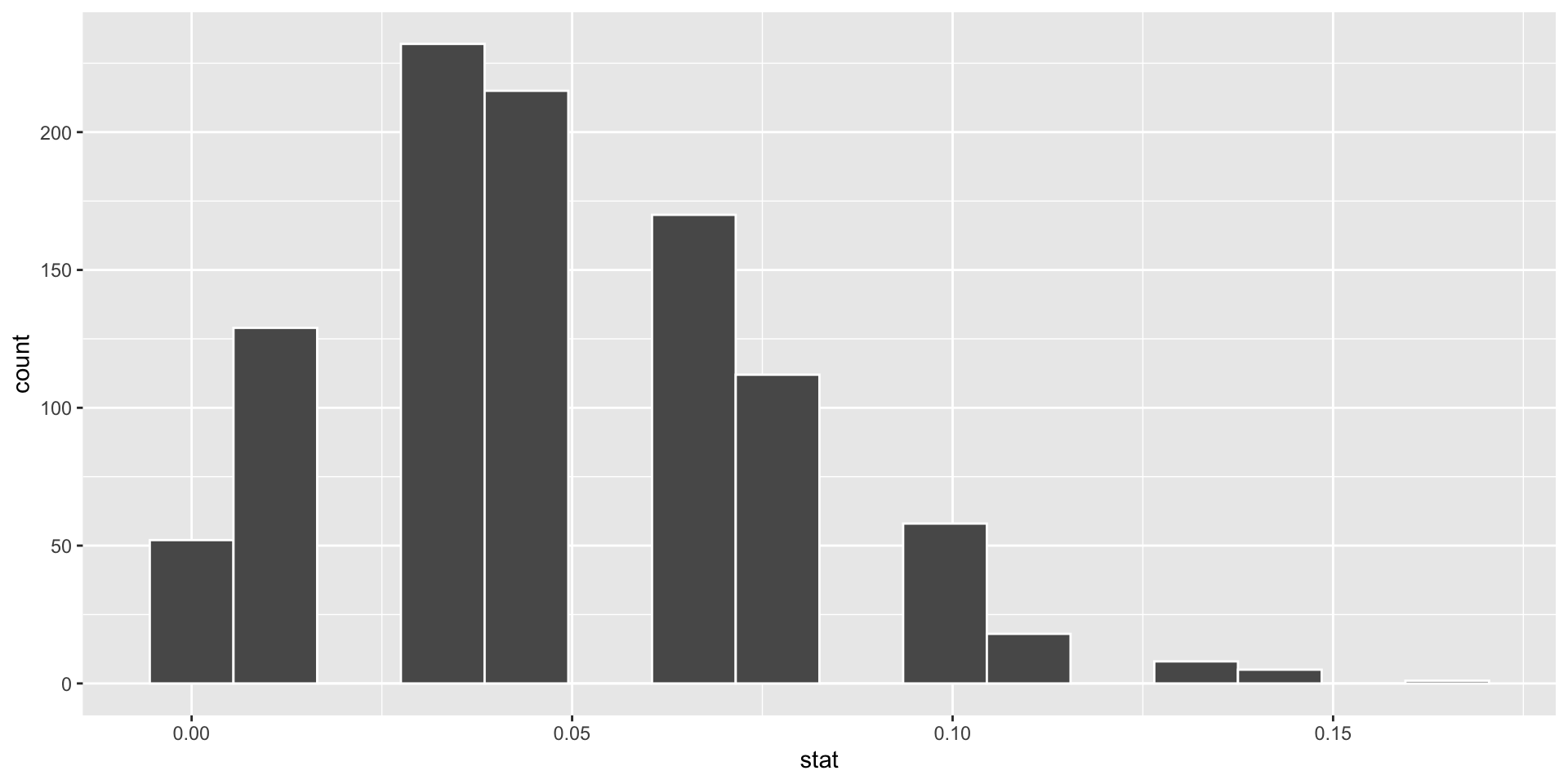
visualize(boot_dist_donor)

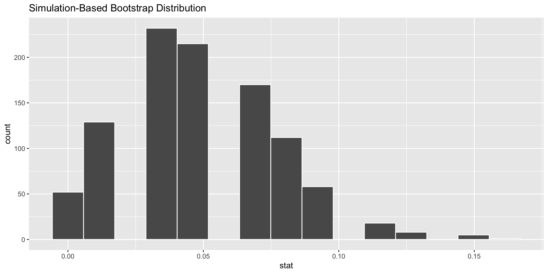
Step 2 – Use Sampling Distribution to get confidence interval

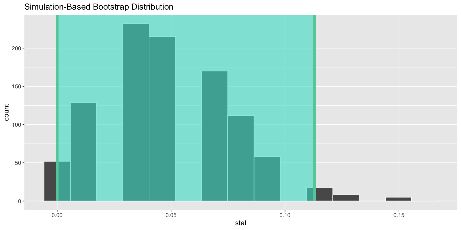
Estimate 95% confidence interval from graph

95% confidence interval

Confidence Interval #2

boot_dist_donor |>
  summarize(
    lower = quantile( stat, 0.025),
    upper = quantile( stat, 0.975)
  )

# A tibble: 1 × 2
  lower upper
  <dbl> <dbl>
1     0 0.113

Confidence Interval #3

ci <- boot_dist_donor |>
  get_confidence_interval(level = 0.95)

ci

# A tibble: 1 × 2
  lower_ci upper_ci
     <dbl>    <dbl>
1        0    0.113

visualize

visualize(boot_dist_donor) +
  shade_confidence_interval(ci)

Interpretation

We are 95% confident that the true proportion is between 0.0 and 0.113.

Notice that this interval contains the national rate of 0.1.

Therefore we cannot be confident (at a 95% level) that true proportion is less than 10%!