AE 06 – Heart Transplants

Application exercise

The Stanford University Heart Transplant Study was conducted to determine whether an experimental heart transplant program increased lifespan. Each patient entering the program was designated an official heart transplant candidate, meaning that they were gravely ill and would most likely benefit from a new heart. Some patients got a transplant and some did not. The variable transplant indicates which group the patients were in; patients in the treatment group got a transplant and those in the control group did not. Of the 34 patients in the control group, 30 died. Of the 69 people in the treatment group, 45 died. Another variable called survived was used to indicate whether the patient was alive at the end of the study. (Turnbull, Brown, and Hu 1974)

Packages and Data

For our analysis, we’ll use the tidyverse and infer packages.

library(tidyverse)
library(infer)

And then, let’s read the data and take a peak at it:

heart_transplant <- read_csv("heart-transplant.csv")
glimpse(heart_transplant)

Rows: 103
Columns: 8
$ id         <dbl> 15, 43, 61, 75, 6, 42, 54, 38, 85, 2, 103, 12, 48, 102, 35,…
$ outcome    <chr> "deceased", "deceased", "deceased", "deceased", "deceased",…
$ transplant <chr> "control", "control", "control", "control", "control", "con…
$ age        <dbl> 53, 43, 52, 52, 54, 36, 47, 41, 47, 51, 39, 53, 56, 40, 43,…
$ survtime   <dbl> 1, 2, 2, 2, 3, 3, 3, 5, 5, 6, 6, 8, 9, 11, 12, 16, 16, 16, …
$ acceptyear <dbl> 68, 70, 71, 72, 68, 70, 71, 70, 73, 68, 67, 68, 71, 74, 70,…
$ prior      <chr> "no", "no", "no", "no", "no", "no", "no", "no", "no", "no",…
$ wait       <dbl> NA, NA, NA, NA, NA, NA, NA, 5, NA, NA, NA, NA, NA, NA, NA, …

The data dictionary is as follows:

Variable	Description
id	ID number of the patient
outcome	Survival status with levels `alive` and `deceased`
transplant	Transplant group with levels `control` (did not receive a transplant) and `treatment` (received a transplant)
age	Age of the patient at the beginning of the study
survtime	Number of days patients were alive after the date they were determined to be a candidate for a heart transplant until the termination date of the study
acceptyear	Year of acceptance as a heart transplant candidate
prior	Whether or not the patient had prior surgery with levels `yes` and `no`
wait	Waiting time for transplant

Heart transplants - `outcome`

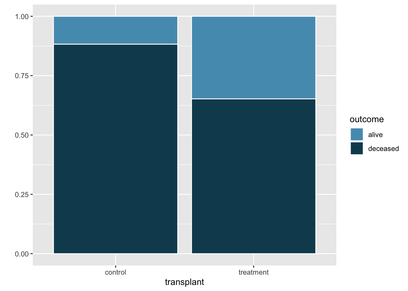
Let’s start by visualizing a possible association between the variables transplant and outcome.

heart_transplant |>
  ggplot( aes(x=transplant, fill = outcome)) +
  geom_bar( position = "fill", color = "white") +
  scale_fill_manual(values = c("#569BBD", "#114B5F")) +
  labs(
    y = ""
  )

Question 1

What does this stacked bar plot tell you (if anything) about a possible association between survival and whether or not the patient got a transplant? Explain your reasoning.

Add your repsonse here

Now let’s calculate the point estimate for the difference in proportions of patients who died between the treatment and control groups. We can express this as \[ \hat{p}_{treatment} - \hat{p}_{control} \] where \(\hat{p}\) is the observed probability of dying in each group.

Question 2

Use the frequency table of outcome by transplant below to calculate the proportions of patients in the treatment and control groups that died? What is the difference in proportions?

Report your results here

heart_transplant |>
  count(transplant, outcome)

# A tibble: 4 × 3
  transplant outcome      n
  <chr>      <chr>    <int>
1 control    alive        4
2 control    deceased    30
3 treatment  alive       24
4 treatment  deceased    45

Another way to do this is to use specify() and calculate() as shown below.

obs_diff_outcome <- heart_transplant |>
  specify(response = outcome, explanatory = transplant, success = "deceased") |>
  calculate(stat = "diff in props", order = c("treatment", "control"))

obs_diff_outcome

Response: outcome (factor)
Explanatory: transplant (factor)
# A tibble: 1 × 1
    stat
   <dbl>
1 -0.230

Question 3

Are the results of this code chunk the same as what you obtained in Question 2?

Add your repsonse here

Question 4

State a null hypothesis and an alternative hypothesis.

Add your repsonse here

The code chunk below generates a null distribution needed to test the hypothesis test you formulated in Question 4. For this simulation we use 100 resamples (reps).

Note: the function set.seed() here is used so that the simulation, although random, is the same everytime it’s run. You can change the seed value to get a different simulation.

# set.seed(2024)

null_dist_outcome <- heart_transplant |>
  specify(response = outcome, explanatory = transplant, success = "deceased") |>
  hypothesize(null = "independence") |>
  generate(reps = 1000, type = "permute") |>
  calculate(stat = "diff in props", order = c("treatment", "control"))

Question 5

Inspect the object null_dist_outcome shown below. How many rows and how many columns does it have? What does each row represent? What does the variable replicate represent? What does stat represent?

Add your repsonse here

print(null_dist_outcome)

Response: outcome (factor)
Explanatory: transplant (factor)
Null Hypothesis: independence
# A tibble: 1,000 × 2
   replicate    stat
       <int>   <dbl>
 1         1 -0.0546
 2         2 -0.0546
 3         3 -0.0985
 4         4  0.0332
 5         5  0.121 
 6         6 -0.0107
 7         7  0.0772
 8         8 -0.142 
 9         9 -0.0107
10        10  0.121 
# ℹ 990 more rows

Now let’s visualize the distribution of simulated differences in proportions of deceased between treatment and control groups.

null_dist_outcome |>
  visualize(bins=14) +
  shade_p_value(obs_stat = obs_diff_outcome, direction = "two-sided")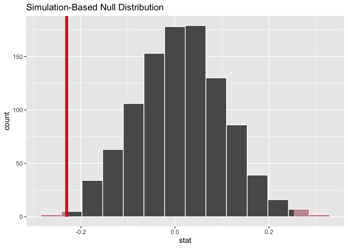

Question 6

What is the shape of this distribution? What is the center of this distribution? What does the red line represent? Are these results expected? Explain your reasoning.

Add your repsonse here

p-value

We can calculate the p-value in two different ways.

Filter null_dist_outcome for stat values that are at least as far away from the null value as the observed value you calculated in Exercise 4. Notice that we are considering both directions!

null_dist_outcome |>
  filter( stat >= 0.23 | stat <= -0.23)

Response: outcome (factor)
Explanatory: transplant (factor)
Null Hypothesis: independence
# A tibble: 16 × 2
   replicate   stat
       <int>  <dbl>
 1       267 -0.230
 2       285 -0.230
 3       311 -0.274
 4       447 -0.230
 5       500  0.253
 6       513  0.253
 7       524  0.297
 8       525 -0.230
 9       653  0.253
10       689  0.253
11       712  0.253
12       720  0.253
13       767  0.253
14       782 -0.230
15       877 -0.274
16       896  0.297

Question 7

Note how many such values there are (rows in the output) and then calculate a proportion using the total number of resamples (i.e. 100).

Add your repsonse here

Use get_p_value():

p_value_outcome <- null_dist_outcome |>
  get_p_value(obs_stat = obs_diff_outcome, direction = "two-sided")

p_value_outcome

# A tibble: 1 × 1
  p_value
    <dbl>
1   0.014

Question 8

Confirm that you obtained the same results with the two methods. Then interpret the p-value in context of the data and the research question and comment on the statistical discernability of this result using a discernability level of 0.05.

Add your repsonse here

Packages and Data

Heart transplants - outcome

p-value

Heart transplants - `outcome`