# A tibble: 4 × 4
# Groups:   gender [2]
  gender decision         n  prop
  <fct>  <fct>        <int> <dbl>
1 male   promoted        21 0.875
2 male   not promoted     3 0.125
3 female promoted        14 0.583
4 female not promoted 10 0.417Hypothesis Testing with Randomization, part two
Chapter 11
In groups
- Discuss Homework: Chapter 11, #3, 5, 7
Gender Discrimination Study
On Tuesday we looked at a study on gender discrimination. The study observed that \(87.5\%\) of male candidates were promoted whereas \(58.3\%\) of female candidates were promoted.
Difference in proportions: \(0.583 - 0.875 = -0.292\)
Test Statistic
State the Hypotheses
\(H_0\) there is no difference between the two groups. Men and women are promoted at the same rate.
\(H_A\) there is a difference. Men are promoted more often than women.
The study observed a difference of \(-0.292\). How unusual would this be if the null hypothesis is true?
If it’s very unusual then we have evidence to reject \(H_0\)
Simulation
- Randomly shuffle a deck of 48 cards that has 35 “promoted” and 13 “not promoted”
- Deal into two groups
- Calculate new difference in proportions
- Repeat!
- Look at the distribution of simulation results
Simulation with R using infer package
specify– what variables are we looking at?hypothesize– what kind of hypothesis test are we doing?generate– do a simulation (many times)calculate– results of the simulation
Visualize results
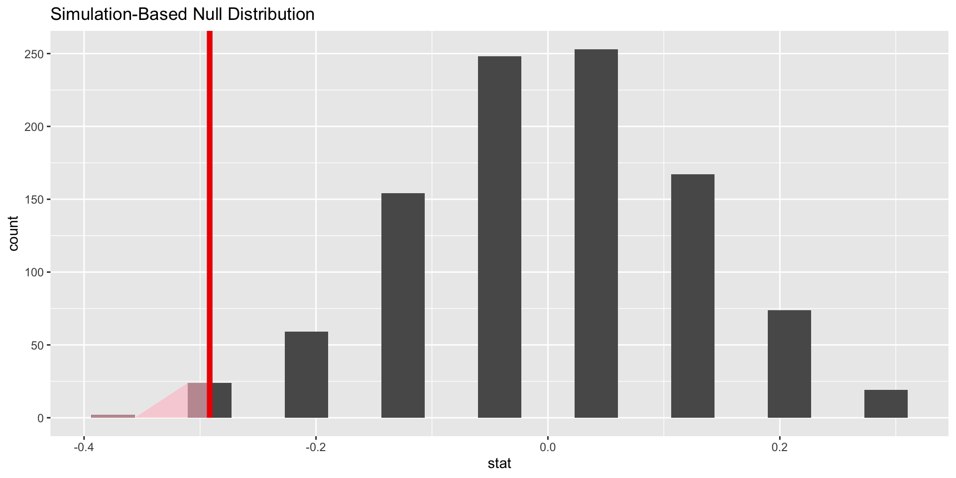
p-value
probability of observing data as (or more) extreme than what we actually got, assuming the null hypothesis is true
In our example, we would want to know how many of the simulated differences were less than or equal to \(-0.29\)
In other words, our observed value of \(-0.29\) happened in the simulations 26 times, or w/ probability \(26/1000 = 0.026\)
Compute p-value with R
# A tibble: 1 × 1
  p_value
    <dbl>
1   0.026
Discernability Level
How much evidence do we require to reject \(H_0\)?
How skeptical are we?
What threshold should we compare p-value to?
Commonly used thresholds (discernability level)
\[
0.1, \, 0.05, \, 0.01
\]
Note: these are also known as significance levels
\(\alpha = 0.05\)
For a discernability level of \(0.05\), we would conclude that since \(p < \alpha\), we have sufficient evidence to reject \(H_0\).
We would say that the data provides statistically discernable evidence against the null hypothesis.
Note: this is often phased as the data being statistically significant
Why \(0.05\)?
A discernability level of \(0.05\) is very common. Why is this?
https://www.openintro.org/book/stat/why05