In Chapters 16 and 17, we looked at proportions measured across two groups - i.e. success and failure
Now, consider variables that have more than two possible options. This means that there is not a single population parameter to look at.
Example: selling used iPad
Seller has a used iPad that is known to have a potential issue (e.g it crashes occasionally)
Buyer provides a prompt: “I’m interested in buying this iPad…”
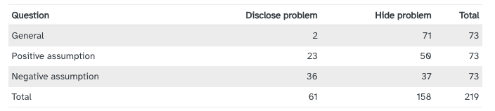
General: … what can you tell me about it?
Positive Assumption: … it doesn’t have any problems, does it?
Negative Assumption: … what problems does it have?
In response to buyer’s prompt, seller either discloses the known issue or does not.
Is there evidence that there the different prompts lead to a difference in disclosure rate?
Is the buyer’s question independent of whether the seller disclosed the problem?
Expected Counts
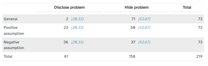
To help us answer this question, we look at expected counts.
If the questions had no impact on what the seller disclosed, we should be able to just look at total number of disclosures out of the total number of cases.
\[
\frac{61}{219} = 0.2785
\]
Then, using this disclosure rate, what would be the expected number of counts in each group?
\[
73 ( 0.2785) = 20.33
\]
\[
73 (1-0.2785) = 52.67
\]
Merry Christmas!
What sound does the “ch” make in the word Christmas?
Why is that?
Chi-squared
For each group we now calculate \[
\frac{( \mbox{observed count} - \mbox{expected count})^2}{\mbox{expected count}}
\] and add them together. This is called the chi-squared test statistic \(\chi^2\).
To decide we look at the chi-squared distribution – same idea as with normal distribution, but different shape.
Use technology (or a table)
The exact shape is determined by the degree of freedom of our two-way table.
Degree of Freedom
\[
df = (\mbox{\# of rows} - 1) \times (\mbox{\# of columns} - 1)
\]
In our example, \[
df = (R - 1)\times (C-1) = 2*1 = 2
\]
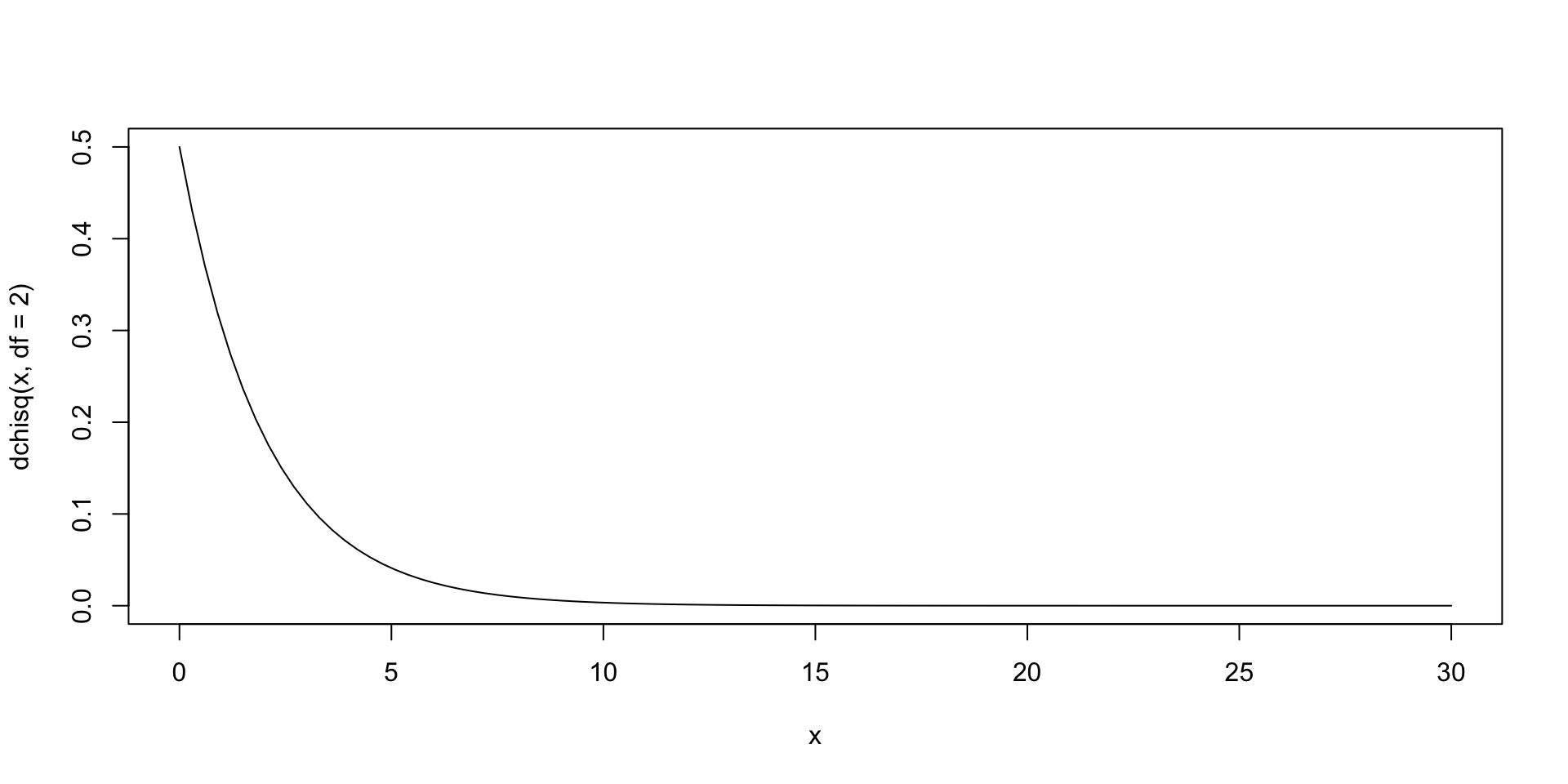
curve(dchisq(x, df =2), from =0, to =30)
1-pchisq(40.13, df =2)
[1] 1.93144e-09
Conclusion
This p-value is very very small! \[
\mbox{p-value} = 0.000000000193
\] Much smaller than our discernment level \(\alpha = 0.05\). We have evidence to reject the null hypothesis.
The data provides convincing evidence that the question asked did affect a seller’s likelihood to tell the truth about problems with the iPad.
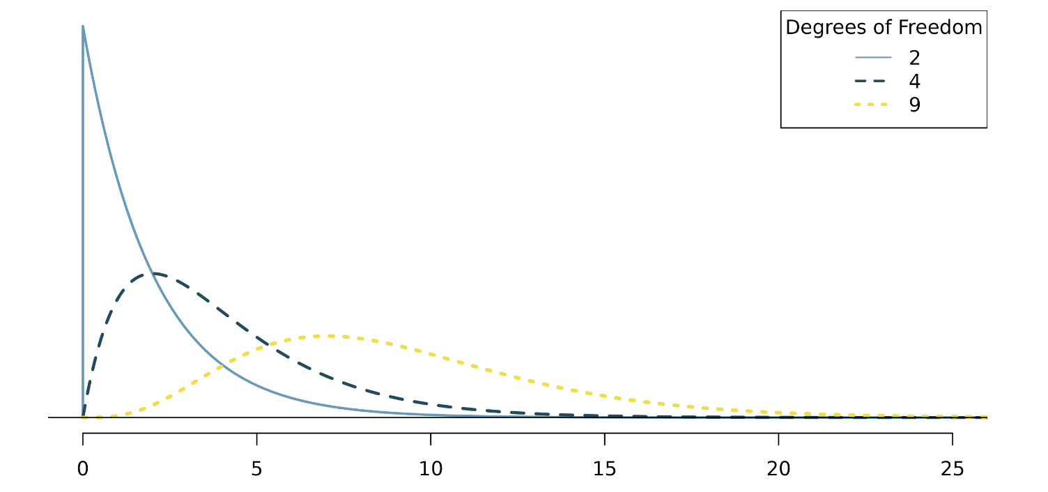
Chi-squared distribution
The larger the degree of freedom, the longer the right tail extends. The smaller the degrees of freedom, the more peaked the mode on the left becomes.
Tools to calculate p-value from a \(\chi^2\) distribution